Remote FPGA verification of DSP algorithm using Red Pitaya Gen2

 Red Pitaya Gen2, Adiuvo Astria
When I was in the university. I remember my FPGA professor saying how important is to simulate our designs. To be honest, in that moment simulations were something boring and I just wanted to get an FPGA development board and test the design in the real hardware (I came from the microcontrollers world). Then, after I started to work with FPGAs, I realized that simulations are not an option, they are a must. However, even simulations are mandatory for every FPGA design, sometimed they are not enough, not because there are non-simulable FPGA desings, but because the FPGA is part of a system that also includes another peripherals like ADCs, DACs, passive elements…
In this article we are going to bring our simulation one step forward, and we are going to test our FPGA design with real analog signals, in a remote way, using a Red Pitaya STEMlab 125-14 Gen2 Pro as signal generator and an Adiuvo Astria Spartan-7 board as the device under test.
We are going to use a Goertzel filter as the DSP algorithm to be verified, but the same setup can be used for any other algorithm or design that needs to be tested with real analog signals. The whole process will be automated with a Python script that will control the Red Pitaya via SCPI, send commands to the FPGA via UART, and generate a test report in Markdown format.
If you have read my earlier articles on the Goertzel algorithm — Single tone detector with Genesys ZU and RTU and Managing AXI4-Stream from MATLAB — you already know the algorithm. This time the twist is different: the Goertzel filter is not the end goal, it is the device under test, and the whole point is to verify it remotely with real analog signals.
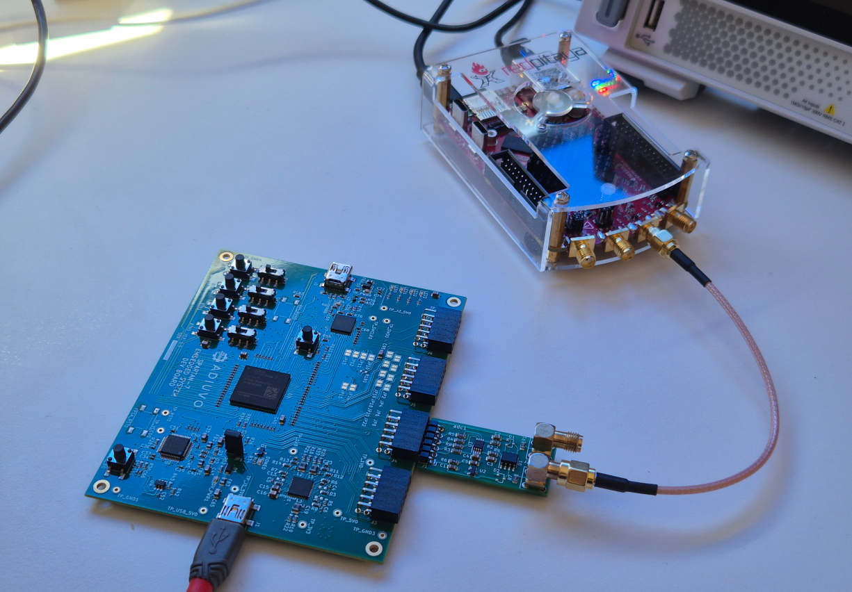
Table of contents
- Why analog-in-the-loop testing matters
- Test setup overview
- The Goertzel filter in Verilog
- ADC acquisition and SPI interface
- UART communication and command protocol
- Controlling the Red Pitaya via SCPI
- The automated Python verification script
- Running the tests and reading the report
- Conclusions
Why analog-in-the-loop testing matters
A well-written Verilog testbench can verify that a digital filter computes the correct output for every input vector you throw at it. What it cannot verify is whether the ADC on your board introduces a DC offset that clips the filter’s accumulator, whether the SPI clock is too fast for the trace length on your PCB, or whether switching noise from the FPGA power supply leaks into the analog input. These are real-world problems that only appear when the complete analog channel is exercised end to end: signal generator, cable, ADC front-end, FPGA fabric, and the communication link back to the host.
This does not mean testbenches are less important — quite the opposite. Testbench simulation is the foundation: it catches logic errors, verifies timing corner cases, and runs in seconds. Analog-in-the-loop testing is the complementary layer on top, the one that catches everything the digital model cannot represent. For safety-critical or production-grade designs, standards like DO-254 and IEC 61508 explicitly require both levels of verification. Even for personal projects, having an automated analog test gives you confidence that a design actually works in the physical world, not just in simulation.
The setup I describe here is deliberately minimal. The goal is to show that you do not need a rack full of instruments or a custom PCB to do meaningful analog-in-the-loop verification — a Red Pitaya, a PMOD ADC, a USB-UART cable, and a Python script are enough to build a useful automated test flow.
Test setup overview
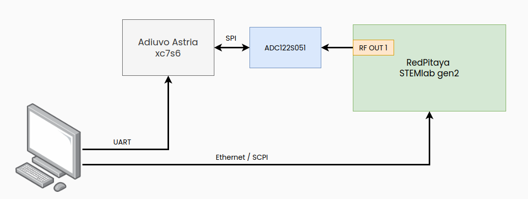
The verification loop involves four physical nodes connected in a closed chain:
- Host PC runs a Python script that orchestrates the entire test.
- Red Pitaya STEMlab 125-14 Gen2 Pro receives SCPI commands over Ethernet (TCP port 5000) and generates sine tones on its OUT1 BNC output.
- ADC PMOD — a custom PMOD carrying a TI ADC122S051 (12-bit, 500 kSPS, SPI interface) — converts the analog signal to digital samples.
- Adiuvo Astria board (Xilinx Spartan-7 XC7S25, synthesized with Vivado 2025.1) runs the Goertzel filter, reads ADC samples via SPI, and communicates results to the host via UART at 115200 baud.
The data flow forms a loop: the Python script tells the Red Pitaya what frequency to generate, tells the FPGA which harmonic to measure, triggers the acquisition, reads back the magnitude result, and decides pass or fail. Then it moves to the next test case. Because the Red Pitaya is controlled over Ethernet and the FPGA over USB-UART, the entire setup can run unattended — or even remotely over SSH.
One thing worth mentioning: the Astria board does not have a built-in USB-UART bridge connected to the FPGA I/O. The board includes an RP2040 co-processor that could be used for this purpose, but for this project I simply connected an external USB-UART adapter to one of the PMOD headers. It is one extra cable, but it keeps the FPGA design independent of the RP2040 firmware.
The Goertzel filter in Verilog
The Goertzel algorithm is a specialized form of the DFT that computes a single frequency bin using a second-order IIR filter. If you need a full derivation, check my earlier article. The key equation is:
\[s[n] = x[n] + 2\cos\left(\frac{2\pi k}{N}\right) \cdot s[n-1] - s[n-2]\]After processing \(N\) samples, the squared magnitude of the \(k\)-th bin is:
\[|X[k]|^2 = s_1^2 + s_2^2 - 2\cos\left(\frac{2\pi k}{N}\right) \cdot s_1 \cdot s_2\]In my previous implementation I computed the real and imaginary parts separately. This time, since the only question the test script needs to answer is “is this frequency bin present or not?”, I compute the squared magnitude directly in the FPGA. I also intentionally omit the cross-term \(2\cos(\cdot) \cdot s_1 \cdot s_2\) from the output. This simplifies the FPGA logic — no extra multiply — and for a pass/fail threshold test, the simplified magnitude \(s_1^2 + s_2^2\) is more than sufficient. If the host ever needs the full magnitude, it can read last_s1 and last_s2 through UART and compute the cross-term in software.
The critical design decision is making the coefficient \(2\cos(2\pi k/N)\) loadable at runtime. The Python script computes the appropriate coefficient for each target harmonic, encodes it in Q2.14 fixed-point format (1 sign bit + 1 bit of integer + 14 fractional bits, range \([-2, +2)\), and sends it over UART. This means a single bitstream can test any frequency bin without resynthesis.
The window size is parameterized as n_samples = 256. With a 50 kHz sample rate, that gives a frequency resolution of approximately 195 Hz — enough to distinguish adjacent test tones separated by 3 bins.
Here is the core of the Goertzel module. The IIR iteration runs on every valid ADC sample, and after \(N\) samples the magnitude is latched and a one-cycle strobe signals the result is ready:
/* Sign-extended sample to accumulator width */
wire signed [acc_width-1:0] sample_ext;

/* Coefficient multiply: coeff_reg * s1, full precision */
wire signed [coeff_width+acc_width-1:0] product;

/* Scaled product: arithmetic right shift to compensate Q format */
wire signed [acc_width-1:0] coeff_s1;

/* IIR next state: s[n] = x[n] + coeff * s[n-1] - s[n-2] */
wire signed [acc_width-1:0] s0;

assign sample_ext = { {(acc_width-sample_width){sample[sample_width-1]} }, sample};
assign product = coeff_reg * s1;
assign coeff_s1 = product >>> coeff_frac_bits;
assign s0 = sample_ext + coeff_s1 - s2;
The always block updates the IIR state on each sample and outputs the magnitude after the window completes:
/* IIR iteration on each valid sample */
if (sample_valid && !compute_mag) begin
  s1 <= s0;
  s2 <= s1;
  if (count == n_samples - 1) begin
    compute_mag <= 1'b1;
  end else begin
    count <= count + 1;
  end
end

/* Magnitude output (one cycle after last sample processed) */
if (compute_mag) begin
  mag <= s1_sq[acc_width-1:0] + s2_sq[acc_width-1:0];
  last_s1 <= s1;
  last_s2 <= s2;
  mag_valid <= 1'b1;
  s1 <= 0;
  s2 <= 0;
  count <= 0;
end
ADC acquisition and SPI interface
The ADC122S051 is a 12-bit, 2-channel successive-approximation ADC from Texas Instruments, rated up to 200 kSPS. Communication is SPI-based: each conversion requires exactly 16 SCLK cycles while CS_n is held low. The channel is selected through bit 11 of the DIN shift register — writing 1 selects IN2, 0 selects IN1. For this project, the Red Pitaya output is connected to IN1 (channel 0), so the control word is always 0x0000.
The SPI master in adc122s051_spi.v generates SCLK at clk / (2 × sclk_div). With a 100 MHz system clock and sclk_div = 4, that gives a 12.5 MHz SPI clock — well within the ADC’s 20 MHz maximum. On every rising SCLK edge, the module shifts out one bit of DIN; on every falling edge, it samples one bit of DOUT. After 16 cycles, the 12-bit result is latched and data_valid pulses for one clock cycle:
if (sclk == 1'b0) begin
  /* Rising edge: shift out DIN */
  din <= shift_out[15];
  shift_out <= {shift_out[14:0], 1'b0};
end else begin
  /* Falling edge: sample DOUT */
  shift_in <= {shift_in[14:0], dout};
  bit_cnt <= bit_cnt + 1;
  if (bit_cnt == BITS_PER_FRAME - 1) begin
    running <= 1'b0;
    cs_n <= 1'b1;
    data <= shift_in[11:0];
    data_valid <= 1'b1;
  end
end
The sample rate is not determined by the SPI clock speed, but by a timer in top.v. A counter divides the 100 MHz system clock down to 50 kHz and pulses adc_start once per period. This ensures the Goertzel filter always receives samples at a known, fixed rate — regardless of how fast the SPI transaction itself completes.
UART communication and command protocol
The host communicates with the FPGA through a simple binary protocol over UART at 115200 baud (8N1). There are only two commands:
0xC0 <high_byte> <low_byte>— Load the Goertzel coefficient. The two data bytes form a 16-bit signed value in Q2.14 format representing \(2\cos(2\pi k/N)\).0xA0— Start an acquisition window. The FPGA triggers exactly \(N = 256\) ADC conversions, runs the Goertzel iteration on each sample, and when the window completes, sends back 4 bytes with the magnitude squared in big-endian format.
The command processor in top.v is a straightforward state machine:
localparam CMD_COEFF = 8'hC0;
localparam CMD_START = 8'hA0;

case (cmd_state)
  ST_IDLE: begin
    if (rx_valid) begin
      if (rx_data == CMD_COEFF)
        cmd_state <= ST_COEFF_HI;
      else if (rx_data == CMD_START)
        cmd_state <= ST_ACQUIRE;
    end
  end
  ST_COEFF_HI: begin
    if (rx_valid) begin
      coeff_hi <= rx_data;
      cmd_state <= ST_COEFF_LO;
    end
  end
  ST_COEFF_LO: begin
    if (rx_valid) begin
      coeff_data <= {coeff_hi, rx_data};
      coeff_valid <= 1'b1;
      cmd_state <= ST_IDLE;
    end
  end
  // ST_ACQUIRE and ST_SEND_RESULT handle acquisition and 4-byte TX
endcase
The UART TX and RX modules themselves are minimal — 8N1 with no FIFO and no flow control. The RX uses double-register synchronization for metastability protection and samples at mid-bit. This simplicity is deliberate: this is a test interface, not a production data link, and keeping it minimal means less area and fewer things to debug.
Controlling the Red Pitaya via SCPI
The Red Pitaya STEMlab exposes a SCPI (Standard Commands for Programmable Instruments) server over TCP on port 5000. This means any language that can open a socket — Python, MATLAB, LabVIEW, even netcat — can configure the signal generator remotely. For this project I use Python with the pyvisa library, which provides a clean high-level interface and works with any VISA-compatible instrument, not just Red Pitaya.
Before sending any commands, you need to enable the SCPI server on the Red Pitaya — it is disabled by default for security reasons. Open the Red Pitaya web interface, go to Settings, and toggle the SCPI Server on. Once enabled, the instrument listens for TCP connections on port 5000.
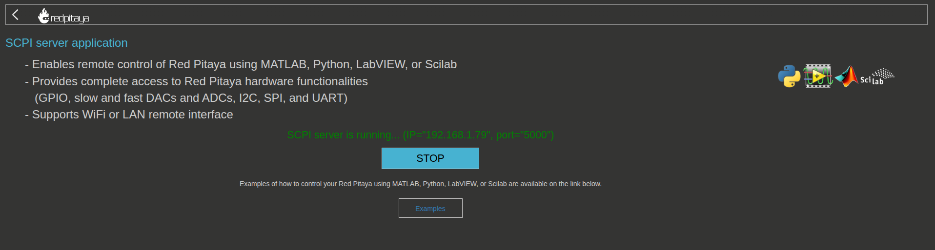
Once the SCPI server is enabled, next time you power cycle the Red Pitaya it will automatically start listening for SCPI commands. You can then connect to it from your Python script and start configuring the signal generator remotely.
Connecting with PyVISA
The first step is opening the SCPI connection. PyVISA wraps the raw TCP socket behind a ResourceManager, and you address the instrument with a VISA resource string:
import pyvisa

IP_ADDRESS = "192.168.100.203"
PORT = 5000

rm = pyvisa.ResourceManager('@py')  # PyVISA-py backend (no NI-VISA needed)
rp = rm.open_resource(
    'TCPIP::{}::{}::SOCKET'.format(IP_ADDRESS, PORT),
    read_termination='\r\n',
    write_termination='\r\n'
)
Pay special attention to the read_termination and write_termination parameters (took me some time to find out why Red Pitaya was not following my instructions). Red Pitaya’s SCPI server expects each command to end with \r\n (carriage return + line feed), and also terminates its responses the same way. Without these two lines, pyvisa will not append the correct terminator when sending commands, and the Red Pitaya will silently ignore them or buffer incomplete data. With the correct terminators set, you can now send SCPI commands and receive responses as expected.
Generating a sine wave
Once the connection is established, configuring the signal generator is straightforward. The SCPI commands follow a consistent hierarchy: SOUR1 for channel 1 parameters, OUTPUT1 for the output stage.
rp.write('GEN:RST')             # Reset the generator to a known state
rp.write('SOUR1:FUNC SINE')     # Waveform: sine
rp.write('SOUR1:FREQ:FIX 2000') # Frequency: 2 kHz
rp.write('SOUR1:VOLT 1.0')      # Amplitude: 1 Vpp
rp.write('SOUR1:TR:INT')        # Trigger immediately (internal trigger)
rp.write('OUTPUT1:STATE ON')    # Enable the physical output
The SOUR1:TR:INT command is essential. On the Red Pitaya Gen2 firmware, configuring the waveform parameters does not start the output by itself — you need to explicitly trigger the generator. Internal trigger mode (TR:INT) tells the instrument to begin generating immediately, without waiting for an external trigger signal. This also applies when you change parameters on the fly: after updating the frequency or amplitude, you must re-send SOUR1:TR:INT for the new configuration to take effect. Without this step, the output will keep running with the old parameters even though the SCPI commands appeared to succeed.
Frequency sweep for oscilloscope verification
Before integrating the Red Pitaya into the automated test pipeline, it is useful to verify that the generator is actually working by observing the output on an oscilloscope. A simple frequency sweep is perfect for this: you can see the signal moving across the screen and confirm that the amplitude stays stable and the frequency changes smoothly.
The following snippet sweeps from 1 kHz to 30 kHz over 10 seconds. Notice how SOUR1:TR:INT is sent after every frequency update — this is the key detail that makes the sweep actually work:
import numpy as np
from time import sleep
import pyvisa

IP_ADDRESS = "192.168.100.203"
PORT = 5000

rm = pyvisa.ResourceManager('@py')  # PyVISA-py backend (no NI-VISA needed)
rp = rm.open_resource(
    'TCPIP::{}::{}::SOCKET'.format(IP_ADDRESS, PORT),
    read_termination='\r\n',
    write_termination='\r\n'
)

f_start = 1000.0    # 1 kHz
f_stop  = 30000.0   # 30 kHz
duration = 10.0     # seconds
steps = 100

freqs = np.linspace(f_start, f_stop, steps)
step_time = duration / steps

# Initial setup
rp.write('GEN:RST')
rp.write('SOUR1:FUNC SINE')
rp.write('SOUR1:VOLT 1.0')
rp.write('SOUR1:FREQ:FIX {}'.format(freqs[0]))
rp.write('OUTPUT1:STATE ON')
rp.write('SOUR1:TR:INT')

# Sweep loop
for freq in freqs:
    rp.write('SOUR1:FREQ:FIX {}'.format(freq))
    rp.write('SOUR1:TR:INT')  # Re-trigger to apply the new frequency
    sleep(step_time)

rp.write('OUTPUT1:STATE OFF')
This sweep covers the range where the Goertzel filter will be tested later, so it also serves as a quick sanity check for the BNC cable and the ADC PMOD: connect the Red Pitaya output to a scope probe and verify the signal across the full range.
The same approach — raw sockets instead of pyvisa — is used in the automated test script (remote_verify.py), where a RedPitayaSCPI class sends commands directly over TCP. Both methods work equally well; pyvisa is more convenient for interactive exploration, while raw sockets avoid the VISA dependency.
The automated Python verification script
The test strategy is built around a three-tone test for each target harmonic \(k\). For every value of \(k\) the script wants to verify, it runs three sub-tests:
- Below tone — Generate a sine at bin \(k-3\) (three bins below the target). The Goertzel filter should report a low magnitude, confirming frequency rejection.
- Target tone — Generate a sine at exactly bin \(k\). The filter should report a high magnitude, confirming detection.
- Above tone — Generate a sine at bin \(k+3\). Again, the filter should report a low magnitude.
This three-point pattern tests both detection and rejection in a single sweep without needing to characterize the full frequency response. A pass/fail threshold separates “high” from “low”.
The coefficient loading function computes \(2\cos(2\pi k/N)\), converts it to Q1.15 fixed-point, and sends the three-byte UART command:
def send_goertzel_coeff(ser: serial.Serial, k: int, n_samples: int):
    """Compute 2*cos(2*pi*k/N) in Q1.15 and send it via UART."""
    coeff = 2.0 * math.cos(2.0 * math.pi * k / n_samples)
    q14 = int(round(coeff * 16384)) # Q2.14 scaling
    q14 = max(-32768, min(32767, q14))
    hi = (q14 >> 8) & 0xFF
    lo = q14 & 0xFF
    ser.write(bytes([CMD_COEFF, hi, lo]))
The test runner function ties everything together, it loads the coefficient, sweeps the three tones through the Red Pitaya via SCPI, triggers an acquisition for each tone, reads back the magnitude, and returns a list of results:
def run_test(rp, ser, target_k, n_samples, sample_rate, amplitude_v, threshold):
    freq_resolution = sample_rate / n_samples
    target_freq = target_k * freq_resolution
    below_freq = (target_k - 3) * freq_resolution
    above_freq = (target_k + 3) * freq_resolution

    tones = [
        ("below", below_freq),
        ("target", target_freq),
        ("above", above_freq),
    ]

    send_goertzel_coeff(ser, target_k, n_samples)

    results = []
    for desc, freq in tones:
        rp_test.set_sine(channel=1, freq_hz=freq, amplitude_v=amplitude_v)
        time.sleep(0.1)
        mag = trigger_acquisition(ser)
        passed = mag > threshold if desc == "target" else mag < threshold
        results.append((desc, freq, mag, passed))
The default test plan sweeps harmonics \(k = 5, 10, 20, 40\), covering target frequencies from about 977 Hz to 7812 Hz at the 50 kHz sample rate. Each harmonic produces three sub-tests, for a total of 12 pass/fail checks per run.
Running the tests and reading the report
Running the full test suite is a single command:
python3 remote_verify.py --rp-ip 192.168.1.79 --serial /dev/ttyUSB0 --report test_report.md
The script connects to the Red Pitaya concurrently with the UART port, runs all test cases sequentially, and prints progress to the terminal as each tone is measured:
Connecting to Red Pitaya at 192.168.1.79....
  Connected.
Opening UART at /dev/ttyUSB0 @ 115200 baud...
  Opened.

=== Test k=5 (target freq = 976.6 Hz) ===
  Coefficient loaded: 2*cos(2π*5/256) = 1.975376
    below   tone @    390.6 Hz → mag² =         312  PASS
    target  tone @    976.6 Hz → mag² =     2845091  PASS
    above   tone @   1562.5 Hz → mag² =         587  PASS

=== Test k=10 (target freq = 1953.1 Hz) ===
  ...
When all tests complete, the script writes a Markdown report file with a summary table, individual results, and the test setup description. This report can be committed to the repository, attached to a pull request, or simply archived for traceability. If you want to run the tests on a schedule — say, after every bitstream build — wrapping the command in a cron job or a CI step is straightforward since the script returns a non-zero exit code on any failure.
Conclusions
I have been working on FPGA-based real time simulators for a while, and the possibilities with these devices are endless. The integration of a Red Pitaya STEMlab gen2 as a signal generator in the test loop is a game-changer for remote verification. It allows you to test your FPGA design with real analog signals without needing physical access to the lab, which is especially valuable in distributed teams or when working from home.
In this project I used a host computer (it can even be a Raspberry PI) to run the python script that orchestrates everything, however if this article has trigger in your mind the idea of building it, you can even run Python script in the Red Pitaya itself. In this case you would need to create your own application using, for example, a Jupyter notebook, and use the Red Pitaya’s GPIO pins to trigger the acquisition instead of sending a command over UART. This would make the setup even more self-contained and portable.