Red Pitaya Gen2: Analysis of an audio signal modulated using PWM

I know Red Pitaya almost since its Kickstarter campaign, and I have been using it for a while now. It is one of those boards that you can bring always with you, actually I have an old one and it came always in my bag. Born as a Kickstarter project back in 2013, it started as an open-source measurement platform built around a Xilinx Zynq SoC, and over the years it has grown into a full ecosystem for test and measurement, SDR, and FPGA development. The Gen2 family is the latest iteration, bringing updated hardware while keeping the same philosophy: a compact, network-connected instrument that you can reprogram at the FPGA level.
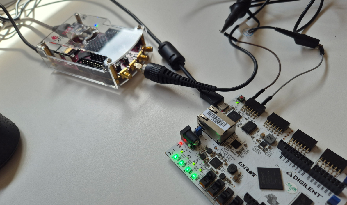
In this article, I want to take a practical look at the Red Pitaya Gen2 by using it as a spectrum analyzer to study a real-world scenario: an audio signal modulated using PWM. PWM audio modulation is the base of Class-D amplifiers, which are widely used in consumer electronics due to their high efficiency. Instead of amplifying the analog waveform directly, a Class-D amplifier encodes the signal as a pulse-width modulated waveform, switches the output stage between the supply rails, and recovers the audio through a low-pass filter. The key trade-off is that the PWM carrier frequency and its harmonics show up in the output spectrum, and the choice of PWM resolution directly determines where that carrier lands. To generate the PWM signal, I am going to use a Digilent Arty A7 board running a simple Verilog modulator at 100 MHz, and I will capture the results with the Red Pitaya’s built-in spectrum analyzer.
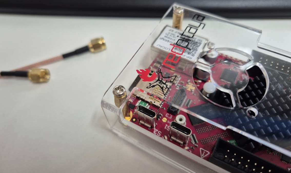
Table of contents
- The hardware inside the Red Pitaya Gen2
- The software ecosystem and workflow
- Custom application development and deployment
- PWM modulation for audio signals
- PWM resolution vs. carrier frequency
- The PWM modulator in Verilog
- Spectrum analysis with the Red Pitaya Gen2
- Conclusions
The hardware inside the Red Pitaya Gen2
The Red Pitaya Gen2 builds on the same core idea as the original STEMlab 125-10: a Xilinx Zynq-7010 SoC paired with high-speed analog front-ends on a compact PCB. The board includes two 125 MSPS ADC channels and two 125 MSPS DAC channels, which give it the bandwidth to work as an oscilloscope, spectrum analyzer, or signal generator up to roughly 50 MHz. The Zynq runs a dual-core ARM Cortex-A9 alongside the FPGA fabric, so there is plenty of room for running Linux, serving web applications, and still having a custom processing pipeline in the PL.
Compared to the original STEMlab, the Gen2 brings some improvements in the analog front-end, with better noise performance, updated board layout, and some connectivity improvements. From my point of view, Red Pitaya is just in the gap between an Analog Discovery and a Zynq development board. With this tool you have a general-purpose Zynq instrument: you get a scope, a spectrum analyzer, a signal generator, and a network analyzer out of the box, but you can also reprogram the FPGA to build your own processing chains. I already covered the first-generation STEMlab in two earlier posts — Getting started with Red Pitaya STEMlab and Custom HW design for Red Pitaya STEMlab — so if you are looking for Vivado project setup details, those are still a good starting point.
The software ecosystem and workflow
One of the things that makes the Red Pitaya stand out is its software stack. When you boot the board, it launches a Linux distribution that starts an Nginx web server. From any browser on the same network, you can access the Red Pitaya’s home page and launch built-in applications: oscilloscope, spectrum analyzer, signal generator, Bode analyzer, and more. There is no need to install desktop software, everything runs in the browser.
Beyond the built-in apps, the Red Pitaya also provides a Jupyter notebook server, which is useful for scripting measurements using Python, and an SCPI server for remote instrument control over TCP. This makes it straightforward to automate test sequences from a host machine using standard SCPI commands, just like you would with a benchtop instrument.
For FPGA developers, the interesting part is that all the built-in applications are open-source and available on GitHub. The web applications are structured as a combination of an FPGA bitstream, a Linux driver or daemon, and a web frontend. This means you can study how the oscilloscope or spectrum analyzer works internally, and use the same framework to build your own applications.
Custom application development and deployment
The Red Pitaya ecosystem supports creating custom web applications that integrate with the FPGA fabric. The official documentation provides a step-by-step guide for building your first web App
The workflow follows a pattern that will be familiar to anyone who has worked with Zynq-based systems: design the PL logic in Vivado, write a C or Python backend that communicates with the FPGA registers through memory-mapped I/O, and build a web frontend using HTML/JavaScript that talks to the backend. The Red Pitaya SDK packages all of this into a deployable application that shows up on the board’s home page alongside the built-in tools.
This approach is particularly useful when you want to create a custom measurement instrument or a demo for a specific signal processing algorithm. You design the DSP pipeline in the FPGA, expose the control registers, and then build a browser-based UI that lets anyone interact with the design without needing Vivado or any FPGA knowledge.
PWM modulation for audio signals
Now, let’s talk about the application. Pulse-Width Modulation is a technique for encoding an analog value into a digital signal by varying the duty cycle of a fixed-frequency square wave. When the input signal is large, the pulse is wider; when it is small, the pulse is narrower. The average value of the PWM waveform, after low-pass filtering, reconstructs the original analog signal.
In the context of audio, PWM is the operating principle behind Class-D amplifiers. Unlike Class-A or Class-AB amplifiers, where the output transistors operate in their linear region and dissipate significant power as heat, a Class-D amplifier switches the output stage fully on or fully off. Since the transistors are either saturated or cut off, the theoretical efficiency approaches 100%. In practice, switching losses bring it down to 85-95%, which is still far better than the 25-50% typical of linear amplifiers. This is why almost every modern portable speaker, laptop, and smartphone uses a Class-D output stage.
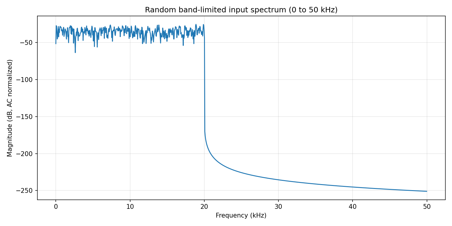
The trade-off is that the PWM carrier and its harmonics appear in the output spectrum. A well-designed low-pass filter removes most of this energy, but the placement of the carrier frequency matters: it must be high enough to stay well above the audio band (20 Hz - 20 kHz) so the filter can attenuate it effectively without affecting the audio content.
PWM resolution vs. carrier frequency
In an FPGA implementation, a counter-based PWM generator divides the system clock by \(2^N\), where \(N\) is the resolution in bits. The PWM carrier frequency is therefore:
\[f_{PWM} = \frac{f_{CLK}}{2^N}\]Since the Arty A7 FPGA runs at 100 MHz, the carrier frequency depends directly on the chosen resolution:
| Resolution | Carrier frequency | Ratio to audio band (20 kHz) |
|---|---|---|
| 8-bit | 390.625 kHz | ~19.5x |
| 9-bit | 195.312 kHz | ~9.8x |
| 10-bit | 97.656 kHz | ~4.9x |
Higher resolution gives finer amplitude granularity, which reduces quantization noise, but it pushes the carrier frequency closer to the audio band. At 10-bit resolution, the carrier sits at only ~97.6 kHz, which is less than 5x the audio bandwidth. This makes filter design harder and can introduce audible artifacts if the filter roll-off is not steep enough.
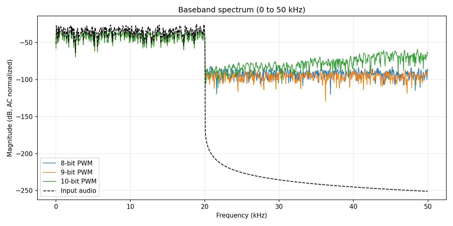
In the following image, we can see a comparison of the spectrum of the PWM signal at 8-bit, 9-bit, and 10-bit resolution. While the spectral content in the audio band looks similar across all three, the carrier fundamental and its harmonics shift downward as resolution increases.
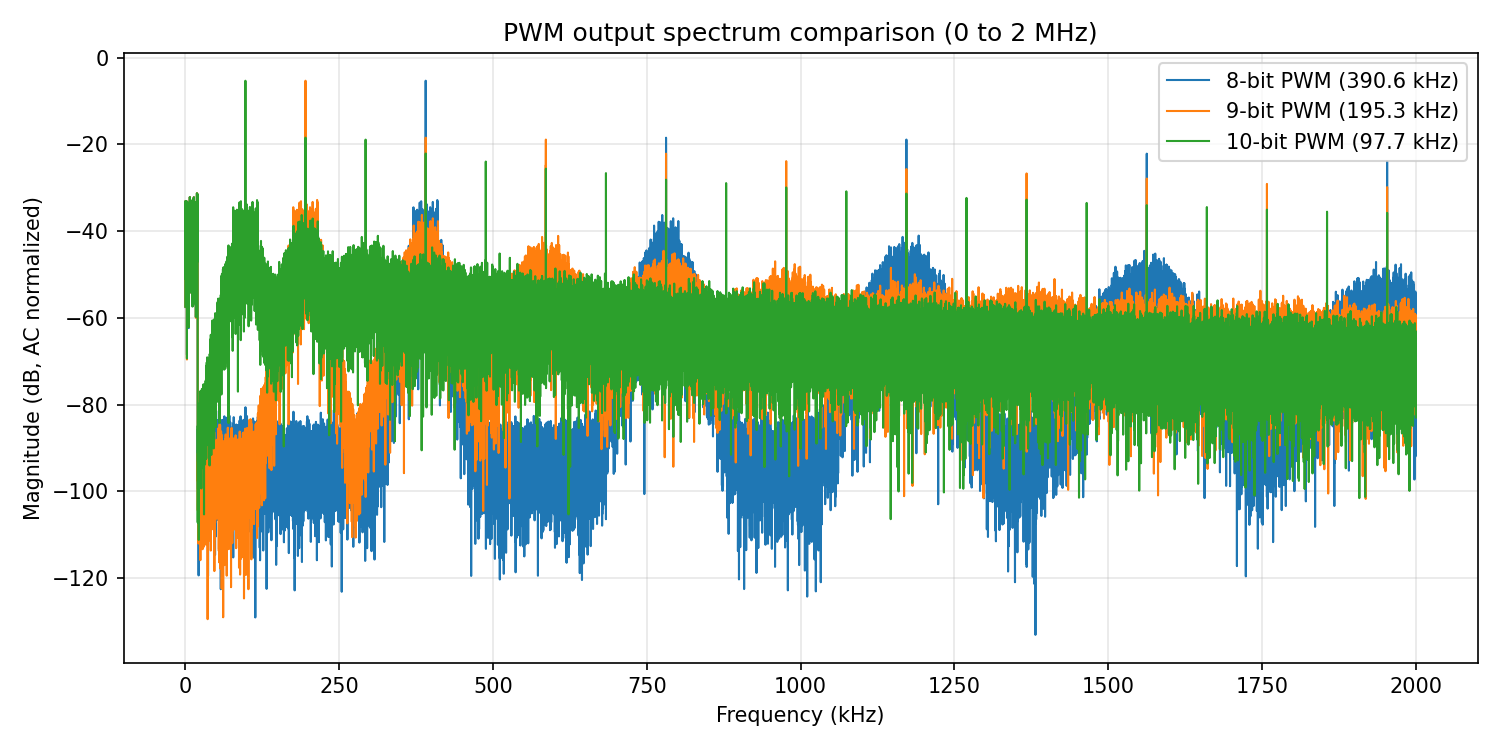
Zooming out to 2 MHz, the harmonic structure becomes even more apparent. The 8-bit signal concentrates its energy at higher frequencies, making it easier to filter, while the 10-bit signal spreads spectral energy closer to the audio band.
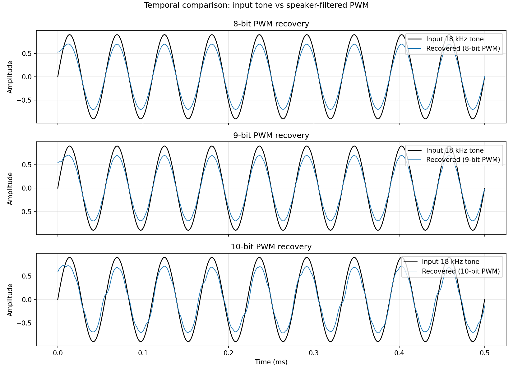
Even though the spectrum may look acceptable, the time-domain signal tells a different story. At lower carrier frequencies, the PWM steps are coarser relative to the audio waveform, and the reconstructed signal after filtering shows visible distortion. This can be perceived as a roughness or grittiness in the audio output.
The PWM modulator in Verilog
The PWM modulator itself is straightforward. A counter runs from 0 to PRESCALER - 1, and the output is driven high whenever the counter value is less than the duty cycle input. When the counter wraps around, a new PWM period begins. The duty cycle input is updated at the audio sample rate, which in this case is determined by an external signal source feeding a sine wave.
module pwm_modulator #(
    parameter integer PRESCALER = 1000
) (
    input  wire clk,
    input  wire [31:0] duty_cycle,
    output reg  pwm_out
);
    reg [31:0] counter = 32'd0;

    always @(posedge clk) begin
        if (counter >= PRESCALER - 1) begin
            counter <= 32'd0;
        end else begin
            counter <= counter + 1;
        end

        pwm_out <= (counter < duty_cycle);
    end
endmodule
For 8-bit resolution, PRESCALER is set to 256, giving a carrier frequency of 390.625 kHz. For 9-bit and 10-bit, the prescaler doubles and quadruples respectively. The duty cycle input maps the audio sample amplitude to the range [0, PRESCALER). In a Class-D amplifier, this mapping would include an offset to center the signal around 50% duty cycle, but for our measurement purposes, a direct mapping is sufficient.
Spectrum analysis with the Red Pitaya Gen2
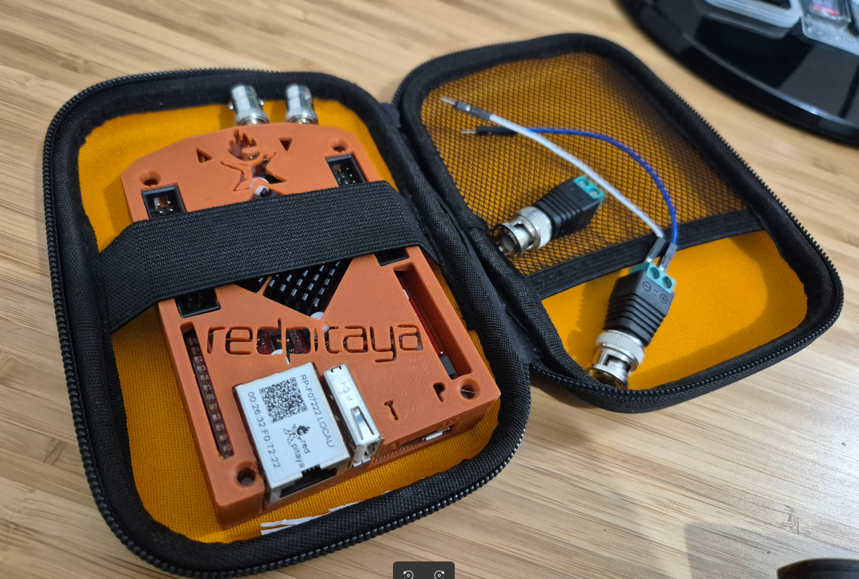
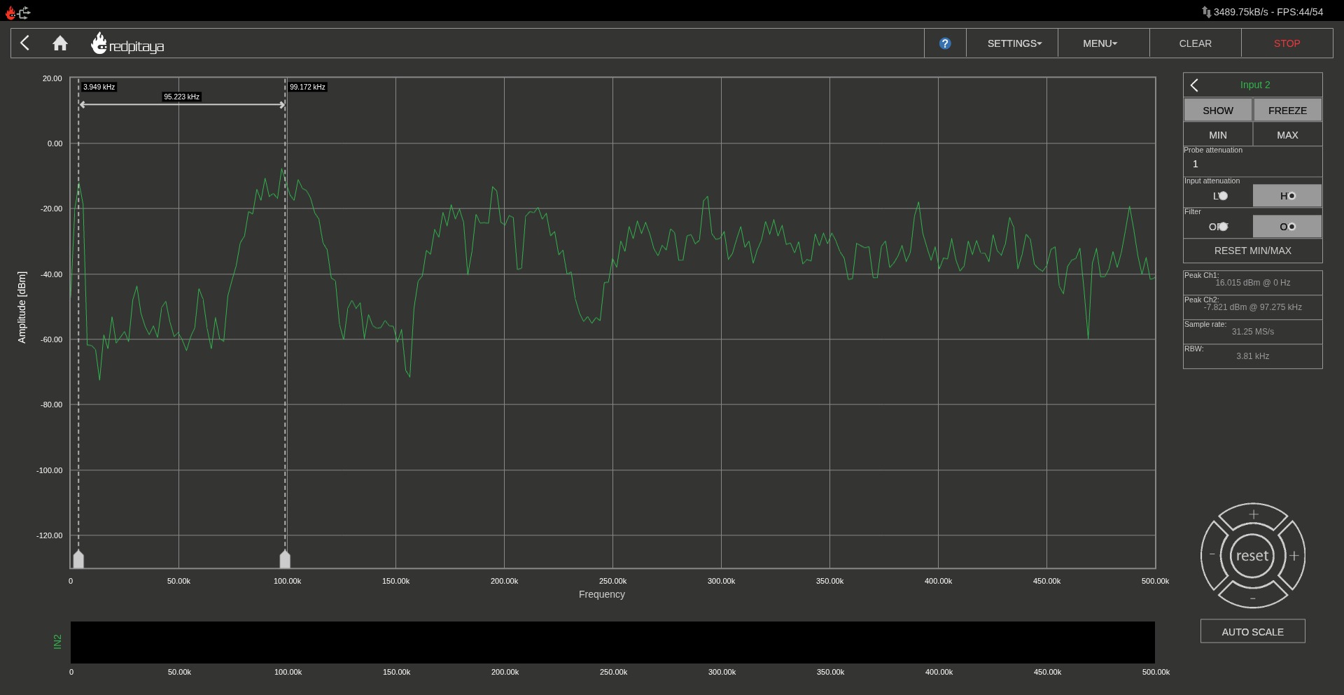
With the PWM modulator running on the Arty A7, I connected its output to the Red Pitaya Gen2’s analog input and used the built-in spectrum analyzer application. The modulating signal is a 3.9 kHz sine wave, which places it well within the audio band and makes it easy to identify in the spectrum.
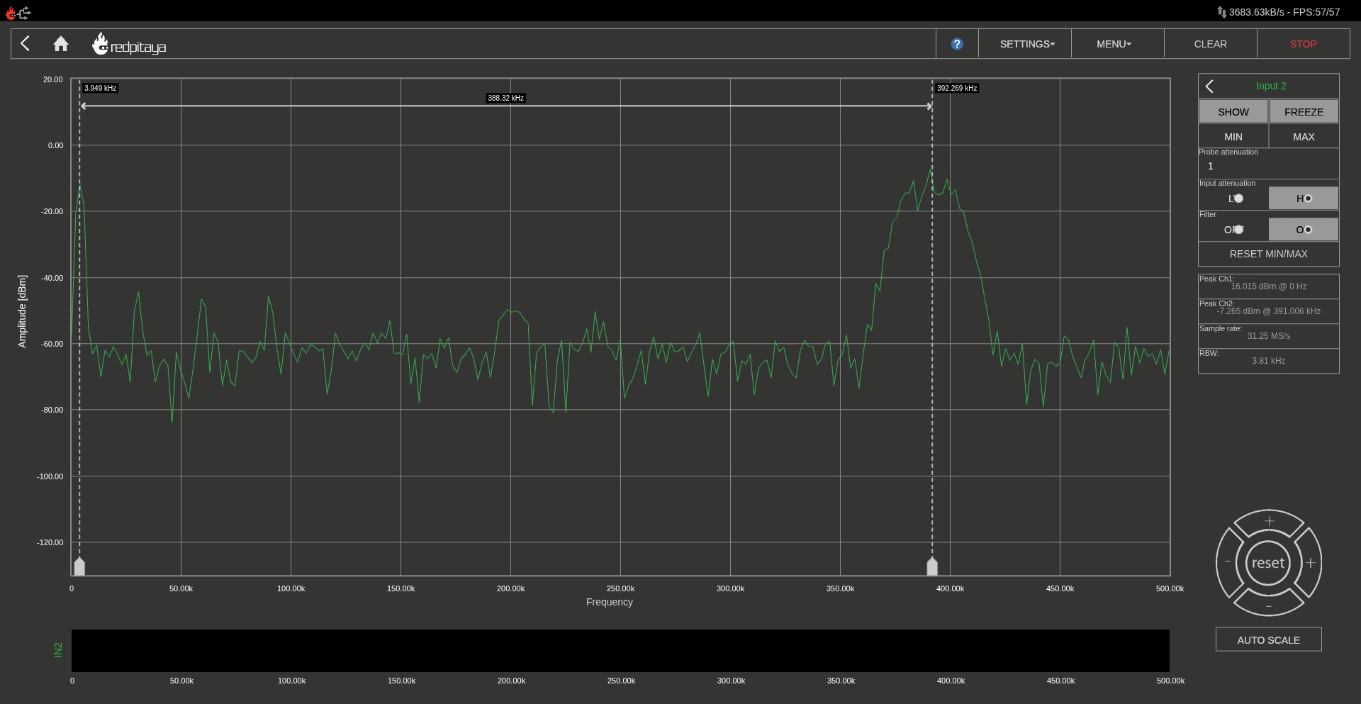
For the 8-bit resolution case (carrier at 390.625 kHz), the spectrum shows the 3.9 kHz fundamental clearly, with the PWM carrier and its harmonics well separated from the audio tone. The first harmonic of the carrier sits at ~781 kHz, far above the audio range.
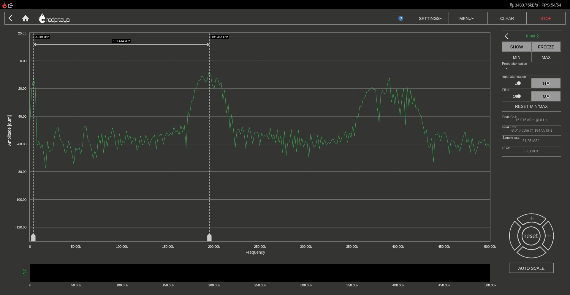
With 9-bit resolution (carrier at 195.312 kHz), everything shifts downward. The carrier is still above the audio band, but its harmonics start to fill in the mid-frequency range. A simple first-order RC filter would struggle to attenuate the carrier sufficiently without affecting frequencies near the top of the audio band.
Finally, with 10-bit resolution (carrier at 97.656 kHz), the carrier fundamental is only about 5x the audio bandwidth. While this gives us finer amplitude resolution (1024 levels instead of 256), the proximity of the carrier to the audio band means that any practical output filter will need a steeper roll-off, typically a second-order or higher LC filter. In a real Class-D design, this is the classic trade-off: more bits give you lower distortion from quantization, but demand a more aggressive output filter.
Conclusions
As I mentioned when I wrote about the Red Pitaya Gen1, the Gen2 is a great tool if you are a scientist, engineer, or hobbyist who wants a compact, network-connected instrument that can be reprogrammed at the FPGA level. In addition, if you are also an FPGA designer, you will get in addition a platform with a SoC, and a high speed ADC and DAC, which can be used to build your own custom measurement instruments. The built-in applications are a good starting point, but the real value is in the ability to create your own tools that integrate with the FPGA fabric.
Regarding the PWM audio side, this experiment made me to think about creating a complete low-power Class-D amplifier design since, I have power transistors and a speaker at home, and I have never tried to build one. I need to make some simulations with different filters and see how the spectrum changes with different PWM resolutions. The Red Pitaya Gen2 would be a great tool to analyze the spectrum of the output signal and compare it with the theoretical predictions.
For now, I have another pending articles about the Red Pitaya Gen2, where I want to explore its capabilities when it is used as an FPGA platform.