Why hardware models can beat software mocks: SPI INA239 and robot arm models

This week I gave a talk in a SW quality meetup. The talk was focused on a practical idea: when we develop software that must communicate with hardware, a hardware model implemented in FPGA can be more useful than a simple software mock.
A software mock is still valuable in early stages, but it usually hides timing and protocol details that become critical in real systems. With an FPGA model, the Linux side sees a real peripheral transaction. That means we can validate not only register-level behavior, but also integration issues related to the hardware environment (for example SPI clocking and transaction timing).
I presented two examples. The first one was an SPI power meter model compatible with INA239 commands. The second one was a robot arm model, where I implemented a quantized biquad filter in FPGA and compared it against the continuous-time motor equation.
Table of contents
- Motivation and talk objective
- Example 1: SPI power meter model compatible with INA239
- SPI slave and command-response controller
- Why this is better than a pure software mock for Linux testing
- Example 2: Robot arm model from continuous equation to FPGA
- Motor equation and discretization
- Biquad implementation and fixed-point interface
- Continuous vs discretized and quantized response
- Build and run flow used in the meetup
- Conclusions
Motivation and talk objective
In real projects, the software team often starts with a lightweight mock because it is fast to create. The problem appears later: once software moves to real hardware, timing assumptions break, edge cases appear, and debugging becomes expensive.
The objective of this talk was to show a middle path: create hardware models that are simple enough to iterate quickly, but realistic enough to exercise protocol behavior as Linux will see it in deployment.
Example 1: SPI power meter model compatible with INA239
The first demo was an SPI power meter. Instead of talking to a physical INA239 chip, Linux talks to an RTL model that implements the same command/response style and key register map.
The model is implemented as an SPI slave plus a controller that decodes commands and returns values for registers like VSHUNT, VBUS, CURRENT, POWER, and DEVICE_ID. I also added simulation registers to inject values and test software behavior deterministically.
To make the model useful for software development, I implemented a concrete subset of the INA239 map plus a few simulation-only registers:
| Address | Acronym | Register Name | Size | Notes |
|---|---|---|---|---|
0x00 |
CONFIG |
Configuration | 16 bits | Includes reset and ADCRANGE behavior |
0x01 |
ADC_CONFIG |
ADC Configuration | 16 bits | Not supported |
0x02 |
SHUNT_CAL |
Shunt Calibration | 16 bits | Not supported |
0x04 |
VSHUNT |
Shunt Voltage | 16 bits | Driven from simulation input |
0x05 |
VBUS |
Bus Voltage | 16 bits | Driven from simulation input |
0x06 |
DIETEMP |
Die Temperature | 16 bits | Driven from simulation input |
0x07 |
CURRENT |
Current Result | 16 bits | Signed (2’s complement) |
0x08 |
POWER |
Power Result | 24 bits | Unsigned |
0x0B |
DIAG_ALRT |
Diagnostic/Alert | 16 bits | Alert flags modeled |
0x0C |
SOVL |
Shunt Overvoltage Limit | 16 bits | Implemented |
0x0D |
SUVL |
Shunt Undervoltage Limit | 16 bits | Implemented |
0x0E |
BOVL |
Bus Overvoltage Limit | 16 bits | Implemented |
0x0F |
BUVL |
Bus Undervoltage Limit | 16 bits | Implemented |
0x10 |
TEMP_LIMIT |
Temperature Limit | 16 bits | Implemented |
0x11 |
PWR_LIMIT |
Power Limit | 16 bits | Implemented |
0x3E |
MANUFACTURER_ID |
Manufacturer ID | 16 bits | Fixed to 0x5449 |
0x3F |
DEVICE_ID |
Device ID | 16 bits | Fixed to 0x2390 |
0x20 |
SIM_VSHUNT |
Simulation VSHUNT Input | 16 bits | Model-only register |
0x21 |
SIM_VBUS |
Simulation VBUS Input | 16 bits | Model-only register |
0x22 |
SIM_DIETEMP |
Simulation DIETEMP Input | 16 bits | Model-only register |
SPI slave and command-response controller
The essential behavior is explicit register addressing and deterministic response generation. The core of the RTL model is:
localparam ADDR_CONFIG          = 6'h00;
localparam ADDR_VSHUNT          = 6'h04;
localparam ADDR_VBUS            = 6'h05;
localparam ADDR_CURRENT         = 6'h07;
localparam ADDR_POWER           = 6'h08;
localparam ADDR_DIAG_ALRT       = 6'h0B;
localparam ADDR_DEVICE_ID       = 6'h3F;
localparam ADDR_SIM_VSHUNT      = 6'h20;
localparam ADDR_SIM_VBUS        = 6'h21;
localparam ADDR_SIM_DIETEMP     = 6'h22;
assign spi_reg_to_send =  (command_byte[7:2] == ADDR_CONFIG)? {reg_config, 8'd0}:
                            (command_byte[7:2] == ADDR_ADC_CONFIG)? {reg_adc_config, 8'd0}:
                            (command_byte[7:2] == ADDR_SHUNT_CAL)? {reg_shunt_cal, 8'd0}:
                            (command_byte[7:2] == ADDR_VSHUNT)? {reg_sim_vshunt, 8'd0}:
                            (command_byte[7:2] == ADDR_VBUS)? {reg_sim_vbus, 8'd0}:
                            (command_byte[7:2] == ADDR_DIETEMP)? {reg_sim_dietemp, 8'd0}:
                            (command_byte[7:2] == ADDR_CURRENT)? {reg_current, 8'd0}:
                            (command_byte[7:2] == ADDR_POWER)? reg_power:
                            (command_byte[7:2] == ADDR_DIAG_ALRT)? {reg_diag_alrt, 8'd0}:
                            (command_byte[7:2] == ADDR_SOVL)? {reg_sovl, 8'd0}:
                            (command_byte[7:2] == ADDR_SUVL)? {reg_suvl, 8'd0}:
                            (command_byte[7:2] == ADDR_BOVL)? {reg_bovl, 8'd0}:
                            (command_byte[7:2] == ADDR_BUVL)? {reg_buvl, 8'd0}:
                            (command_byte[7:2] == ADDR_TEMP_LIMIT)? {reg_temp_limit, 8'd0}:
                            (command_byte[7:2] == ADDR_PWR_LIMIT)? {reg_pwr_limit, 8'd0}:
                            (command_byte[7:2] == ADDR_MANUFACTURER_ID)? {MANUFACTURER_ID, 8'd0}:
                            (command_byte[7:2] == ADDR_DEVICE_ID)? {DEVICE_ID, 8'd0}:
                            24'h000000; // Default to 0 for undefined addresses
For the reading side, the SPI slave captures the command byte and then sends the corresponding register value in the next bytes. For writing, it updates internal registers based on the command and data bytes received.
      case (command_byte[7:2]) // Address is bits[7:2]
        ADDR_CONFIG: reg_config <= {data_write_rcv[15:8], data_write_rcv[7:0]};
        ADDR_ADC_CONFIG: reg_adc_config <= {data_write_rcv[15:8], data_write_rcv[7:0]};
        ADDR_SHUNT_CAL: reg_shunt_cal <= {data_write_rcv[15:8], data_write_rcv[7:0]};
        ADDR_SOVL: reg_sovl <= {data_write_rcv[15:8], data_write_rcv[7:0]};
        ADDR_SUVL: reg_suvl <= {data_write_rcv[15:8], data_write_rcv[7:0]};
        ADDR_BOVL: reg_bovl <= {data_write_rcv[15:8], data_write_rcv[7:0]};
        ADDR_BUVL: reg_buvl <= {data_write_rcv[15:8], data_write_rcv[7:0]};
        ADDR_TEMP_LIMIT: reg_temp_limit <= {data_write_rcv[15:8], data_write_rcv[7:0]};
        ADDR_PWR_LIMIT: reg_pwr_limit <= {data_write_rcv[15:8], data_write_rcv[7:0]};
        // Simulation registers
        ADDR_SIM_VSHUNT: reg_sim_vshunt <= {data_write_rcv[15:8], data_write_rcv[7:0]};
        ADDR_SIM_VBUS: reg_sim_vbus <= {data_write_rcv[15:8], data_write_rcv[7:0]};
        ADDR_SIM_DIETEMP: reg_sim_dietemp <= {data_write_rcv[15:8], data_write_rcv[7:0]};
        default: ; // Ignore writes to undefined addresses or read-only registers
      endcase
To integrate this model into Linux, I exposed it as a spidev device. The device tree node for the SPI slave looks like this:
&spi0 {
    status = "okay";
    #address-cells = <1>;
    #size-cells = <0>;

    spidev@0 {
        compatible = "rohm,dh2228fv";
        reg = <0>;                /* Chip select 0 */
        spi-max-frequency = <10000000>;
        status = "okay";
    };
};
On the software side, a minimal spidev application is enough to validate the interface:
def _cmd(self, addr: int, read: bool) -> int:
    cmd = ((addr & self.addr_mask) << self.cmd_shift) & 0xFF
    if read:
        cmd |= (1 << self.rw_bit)
    return cmd

def read_reg16(self, addr: int) -> int:
    tx = [self._cmd(addr, True), 0x00, 0x00]
    rx = self.spi.xfer2(tx)
    return (rx[1] << 8) | rx[2]
Why this is better than a pure software mock for Linux testing
This was the key message of the first demo. For the Linux kernel and user-space driver, the transaction is a real SPI transaction over the platform SPI controller, not a function call to a fake object.
Because of that, you can expose issues that software mocks usually hide: mode mismatches, clock-related behavior, transfer framing assumptions, and other effects linked to the real hardware path.
In other words, you can validate software against a controlled model while still preserving the electrical/protocol context of the real system.
Example 2: Robot arm model from continuous equation to FPGA
The second demo used a robot arm motor model. The starting point is the continuous-time motor equation in the \(s\) domain. From there, I derived a discrete-time form and implemented it as a quantized biquad in FPGA.
This lets software interact with a realistic dynamic response instead of a static or idealized mock value.
Motor equation and discretization
The continuous-time model I used is:
\[\frac{\omega(s)}{V(s)}=\frac{K_t}{(R_a + L_a s)(J s + B)+K_tK_e}\]Using the values from the project:
\(K_t = 0.0274\)
\(K_e = 0.0274\)
\(R_a = 4.0\ \Omega\)
\(L_a = 2.75\times10^{-6}\ H\)
\(J = 15\times10^{-6}\ kg\cdot m^2\)
\(B = 3.5\times10^{-6}\ N\cdot m\cdot s/rad\)
the transfer function becomes:
\[\frac{\omega(s)}{V(s)}= \frac{0.0274} {(4 + 2.75\times10^{-6}s)(15\times10^{-6}s + 3.5\times10^{-6}) + 0.0274^2}\]and after expansion:
\[\frac{\omega(s)}{V(s)}= \frac{0.0274} {4.125\times10^{-11}s^2 + 6.0000009625\times10^{-5}s + 7.6476\times10^{-4}}\]Then I discretized it with Tustin using \(T_s = 100\ \mu s\) and mapped it to the biquad structure implemented in FPGA.
The implemented quantized coefficients were:
\(b_0 = 1475/2^{16} = 0.0225067\)
\(b_1 = 2950/2^{16} = 0.0450134\)
\(b_2 = 1475/2^{16} = 0.0225067\)
\(a_1 = -1694/2^{16} = -0.0258484\)
\(a_2 = -63677/2^{16} = -0.9713898\)
So the discretized transfer function used in hardware is:
\[H(z)=\frac{Y(z)}{X(z)}= \frac{0.0225067 + 0.0450134z^{-1} + 0.0225067z^{-2}} {1 - 0.0258484z^{-1} - 0.9713898z^{-2}}\]and the corresponding difference equation is:
\[y[n] = 0.0225067\,x[n] + 0.0450134\,x[n-1] + 0.0225067\,x[n-2] + 0.0258484\,y[n-1] + 0.9713898\,y[n-2]\]Biquad implementation and fixed-point interface
The FPGA model uses a biquad block and fixed-point I/O. The software writes a command voltage and reads speed through AXI4-Lite/MMIO.
These are the key MMIO/Q16 conversion lines used in the demo scripts:
ADDR_VOLTAGE = 0x80000000
ADDR_SPEED = 0x80000004

def q16_to_float(raw_u32: int) -> float:
    if raw_u32 & 0x80000000:
        raw_s32 = raw_u32 - (1 << 32)
    else:
        raw_s32 = raw_u32
    return raw_s32 / 65536.0

def float_to_q16(value: float) -> int:
    scaled = int(round(value * 65536.0))
    return scaled & 0xFFFFFFFF
This interface is simple enough for quick testing but still representative of a real embedded control path.
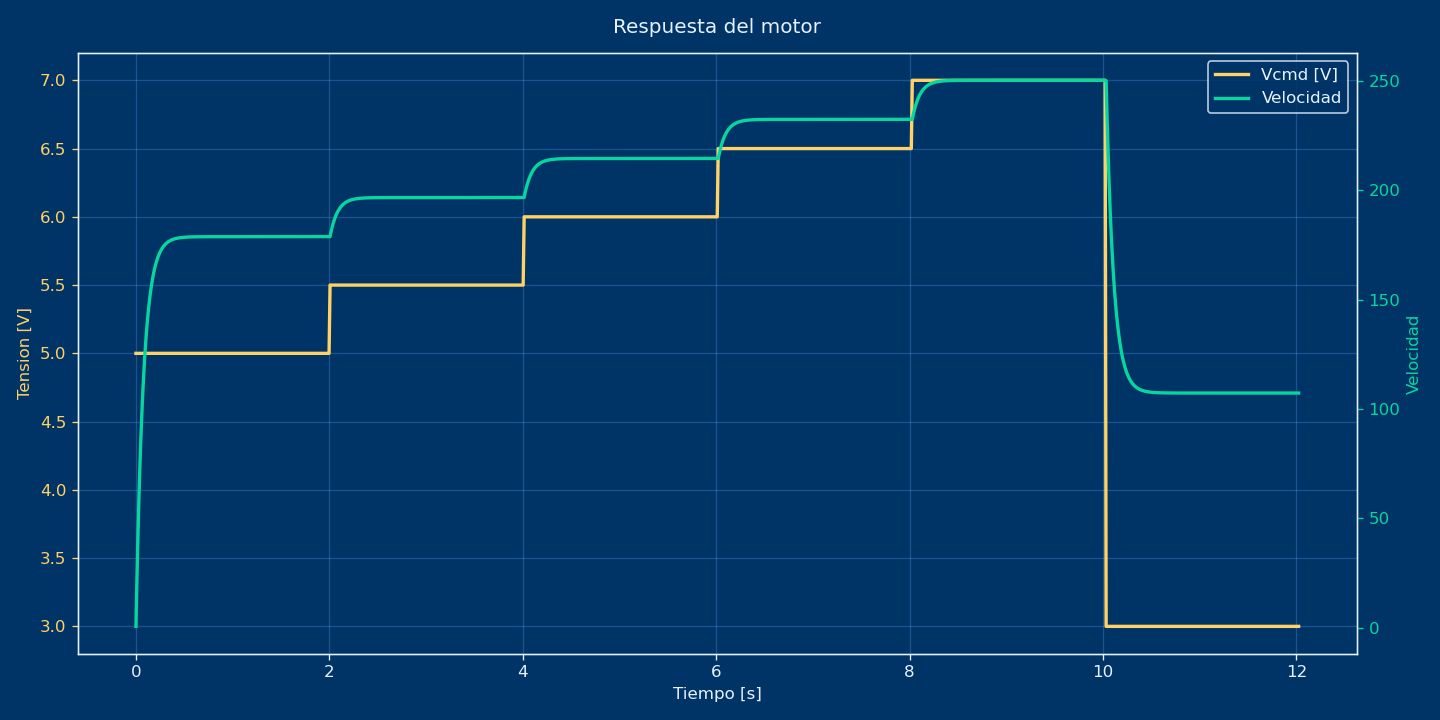
Continuous vs discretized and quantized response
A central point in the talk was comparing three things: the motor response from the continuous equation, the discretized model, and the final quantized implementation running in FPGA.
That comparison is important because it shows exactly what we lose (and what we keep) when moving from mathematical model to digital hardware implementation.

With this comparison, we can justify that the hardware model is realistic enough for software development and integration testing.
Build and run flow used in the meetup
To keep the demo reproducible, I used a scripted Vivado setup and small Python applications.
The essential Vivado Tcl block was:
set project_name "te0802_meetup"
set project_dir script/vivado_projects/$project_name
set rtl_dir rtl/rtl_robot_arm
set xdc_dir xdc

set board_part "trenz.biz:te0802_2cg_1e:2.0"
set part "xczu2cg-sfvc784-1-e"

create_project $project_name $project_dir -part $part -force
set_property board_part $board_part [current_project]
set verilog_files [glob -nocomplain $rtl_dir/*.v]
add_files -fileset sources_1 -norecurse $verilog_files
add_files -fileset constrs_1 -norecurse [glob -nocomplain $xdc_dir/*.xdc]
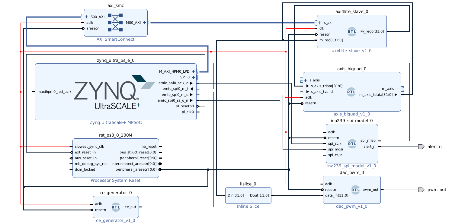
The complete Vivado block design included the SPI slave, the biquad block, AXI4-Lite interfaces, and the INA239 model.
And the command sequence shown during the talk was:
python3 host/ina239_spidev_app.py --bus 0 --device 0 --mode 1 --count 5 --interval 0.2
sudo python3 host/motor_voltage_steps.py --steps 5.0,5.5,6.0,6.5,7.0,3.0 --dwell 1.5 --sample 0.1 --csv host/motor_steps_log.csv
python3 host/plot_motor_csv.py host/motor_steps_log.csv --out host/motor_escalones.png
Conclusions
The meetup thesis was simple: for communication-heavy software development, a hardware model can provide better validation value than a pure software mock.
In the SPI power meter example, Linux sees real SPI transactions, so protocol and timing assumptions are tested in a realistic context. In the robot arm example, the quantized biquad model provides dynamic behavior close to the motor model, making software tests much more meaningful than constant-value stubs.
This approach does not replace all mocks, but it is a strong option when you need early software progress without giving up hardware realism.