Receiving ADS-B (1090 MHz) with a USRP B206mini-i and GNU Radio

Disclaimer: This article is provided for educational and research purposes only. Any signal capture, analysis, or related activity should be performed exclusively in a controlled lab environment and in full compliance with applicable laws and regulations. The author assumes no responsibility or liability for how this information is used, nor for any consequences arising from its application outside of a lawful and authorized context.

Aeronautics is one of the most critical systems we have, and fortunately is one of the most secure means of transport. This is possible due to the high amount of security measures that aircrafts feature, and most of them are completely automatic. An example of one of these features is the Automatic Dependent Surveillance Broadcast[ (ADS-B). This technology allows the aircraft to determine its position via satellite navigation, or other sensors, and periodically broadcast its position and other related data, enabling it to be tracked.

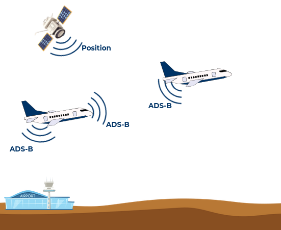
This information is not encrypted, and can be received by air traffic control ground bases, satellite-based receivers and even other aircrafts, so everyone knows the position of the aircraft. As a curiosity, flightradar24 works using this data to locate in the map the position of the aircrafts.

Talking about technical details, ADS-B works by broadcasting frames that contain all the information. This frame is sent in the 1090 MHz band and it is modulated using a simple OOK modulation. In this article we are going to use the new USRP B206mini-i to receive and decode this frames.

The USRP B206mini-i is a portable SDR able to work in a frequency range from 70 MHz to 6GHz, with a bandwidth up to 56 MHz. These features allow the B206mini-i to receive ADS-B frames and using GNURadio and the Python package pyModeS we are going to be able to decoding the frames, and this is exactly what we are going to do in this article.

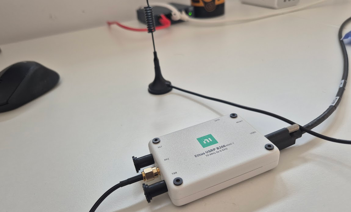
Table of Contents

• Signal Spectrum analysis
• Demodulation
• Saving data in files
• Decoding data
• Decoding Mode-S frame
• Conclusions

Signal Spectrum analysis

First of all, we are going to create a basic GNU Radio flowgraph to capture data and verify that the B206mini-i and the antenna are configured correctly and well located .

The flowgraph include a UHD: USRP Source with a center frequency configured using a variable to 1090 MHz, a sample rate of 5 Msps, and then we need to add QT GUI Frequency Sink, to verify that data is received in the correct frequency and a QT GUI Waterfall Sink that will act as a persistence for the frequency.

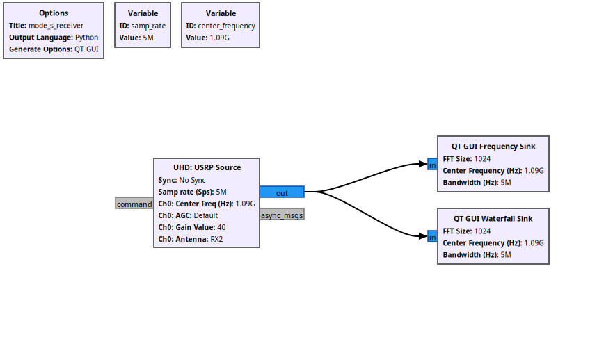
Now, we can compile, connect the SDR to a USB-C port, and run the design to verify if we can receive the frames.

After a couple of seconds, we can check in the waterfall that some frames have been received in the 1090 MHz band, so in principle, the setup is working.

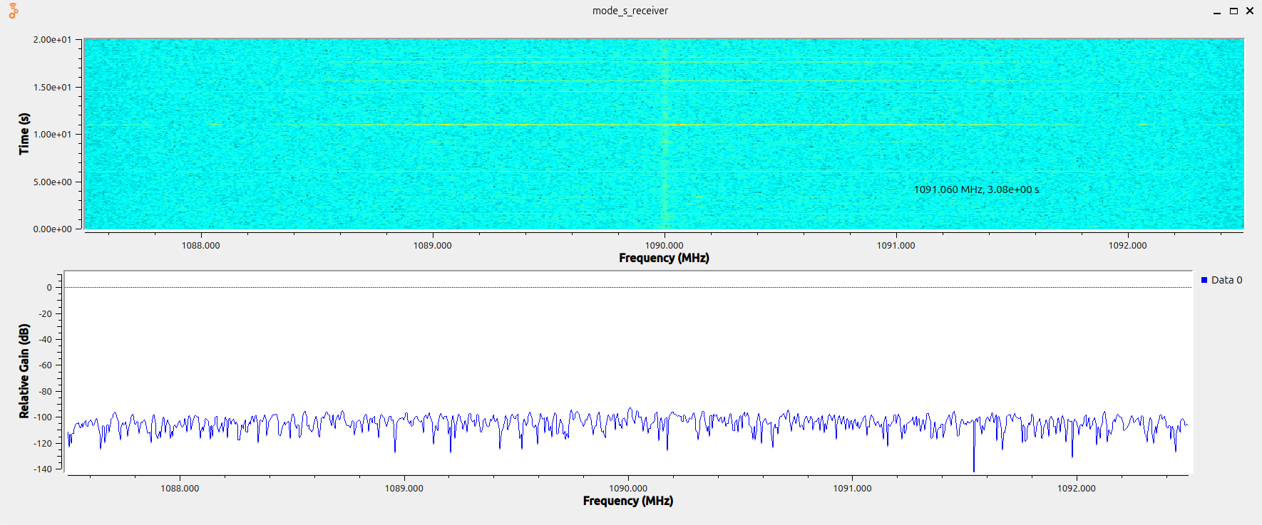
Now, we can demodulate the signal.

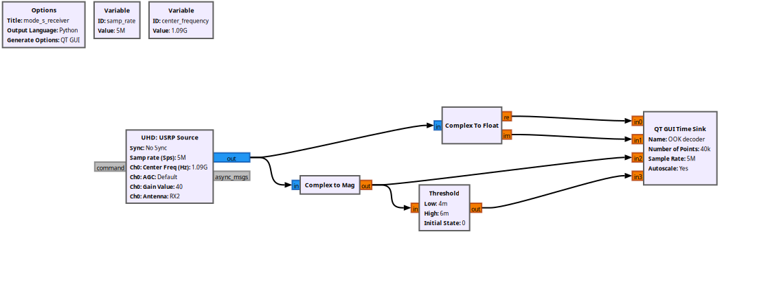
Demodulation

Now we can receive frames, it is time to verify that those frames are correct. To demodulate the signal, since we know that it is modulated using OOK modulation, we can obtain the envelope of the signal by computing the absolute value of the complex signal using the block Complex to Mag. Then using a Threshold block with the values according to the power of the signal received we will obtain the binary data of the frame. Then in order to visualize the data, we can include a QT GUI Time Sink to see the frames received.

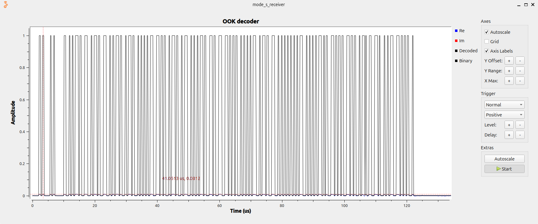
The ADS-B frame format is based on a preamble of 8us where for 1s are sent, and then 56 to 112 us of data with a bitrate of 1 Mbit/second.

In the next image we can find the preamble, and then the data received, that is corresponding with a 112us length frame.

The next step is to save the frames received to decode them in Python.

Saving data in files

Since we want to save in the files only the frame received, we need to detect the frame, open a new file when the frame starts, wait until the frame ends and then close the file. We can do this in GNU Radio using tags. The trigger used to start saving data will be the first rising edge of the demodulated signal, then using a Moving Average filter block, we can hold the trigger the length of the filter. This way, the True value in the output of the filter will be held as long as a ‘1’ is received, plus the length of the filter. This true of False value are connected to a Burst Trigger block, that will act as a switch for the data, allowing the write in a new file only when the trigger input is True.

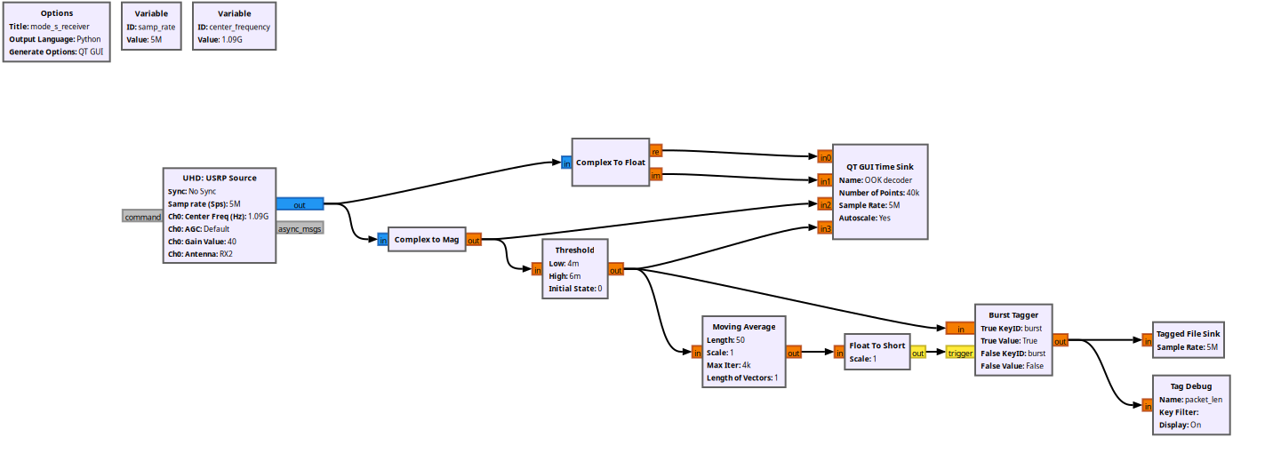
This will generate a set of files. Notice that in the same band, we will find ADS-B frames, but also Mode-S frames so some of the files saved won’t contain the information we need. However, we are going to make this separation in the Python script.

Decoding data

As I mentioned in the introduction of this article, we are going to use the Python package pyModeS. This module needs the hexadecimal data frame of the ADS-B frame to decode it, so we need to obtain these values.

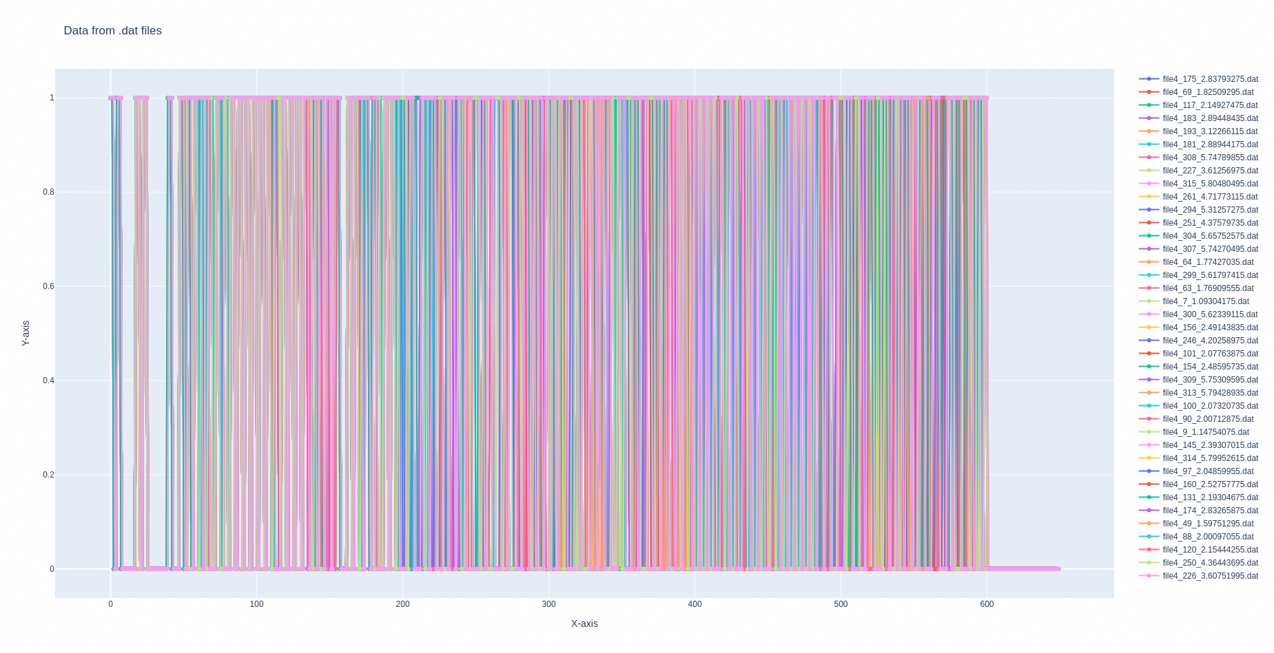
Python next draws the frames received using Plotly. This script applies a decimation factor of 1 just to check whether the signal is well captured or not. Also, the script uses the samples_per_frame variable that calculates the length of the frame, and also plots the frames with a length greater than this value. This way we can reject the rest of the frame.

import numpy as np
import glob
import plotly.graph_objs as go
from plotly.offline import plot

# Decimation factor
decimation_factor = 1

# Mode-S frame length in bits
mode_s_frame_length_bits = 112

# Samples per bit for Manchester decoding
sample_rate = 5e6 # 5 Msps
bit_rate = 1e6 # 1 Mbaud
samples_per_bit = int(sample_rate / bit_rate)

# Calculate the number of samples per Mode-S frame
samples_per_frame = mode_s_frame_length_bits * samples_per_bit

# Search .dat files in the current directory
data_files = glob.glob("*.dat")

# generate plotly traces for each data file
traces = []
for file in data_files:
    data = np.fromfile(open(file), dtype=np.float32)
    
    # Add trace only if data length is sufficient
    if len(data) >= samples_per_frame:
        trace = go.Scatter(
            x=np.linspace(0, len(data)-1, len(data)),
            y=data_decimate,
            mode='lines+markers',
            name=file
        )
        traces.append(trace)
# Create layout for the plot
layout = go.Layout(
    title='Data from .dat files',
    xaxis=dict(title='X-axis'),
    yaxis=dict(title='Y-axis'),
)
fig = go.Figure(data=traces, layout=layout)

# Save the plot as an HTML file
plot(fig, filename='data_plot.html')

The next figure shows all the ADCS-B frames with a duration of 112us.

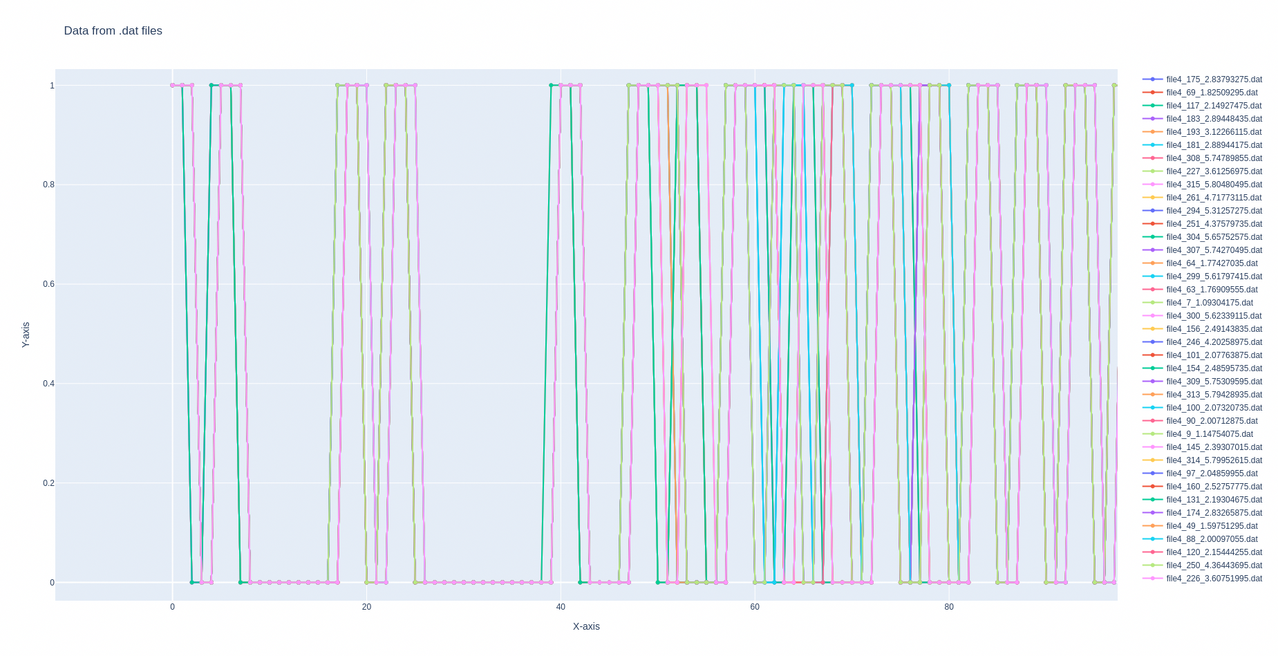
If we take a look at the preamble, we can see that even though they are very well synchronized, we can move some of them into one sample to make a better synchronization. This is done by verifying the first 8 bits of the frame.

def synchronize_data(data):
    data = np.asarray(data)
    # Normalize data
    bits = (data > 0).astype(np.uint8)

    p1 = np.array([1,1,1,0,0,1,1,1], dtype=np.uint8)
    p2 = np.array([1,1,0,0,1,1,1,0], dtype=np.uint8)

    if bits.size >= 8 and np.array_equal(bits[:8], p2):
        out = np.concatenate((np.array([1.0], dtype=np.float32),
                              data.astype(np.float32)))
        return out
    elif bits.size >= 8 and np.array_equal(bits[:8], p1):
        return data.astype(np.float32)
    else:
        # default
        return data.astype(np.float32)

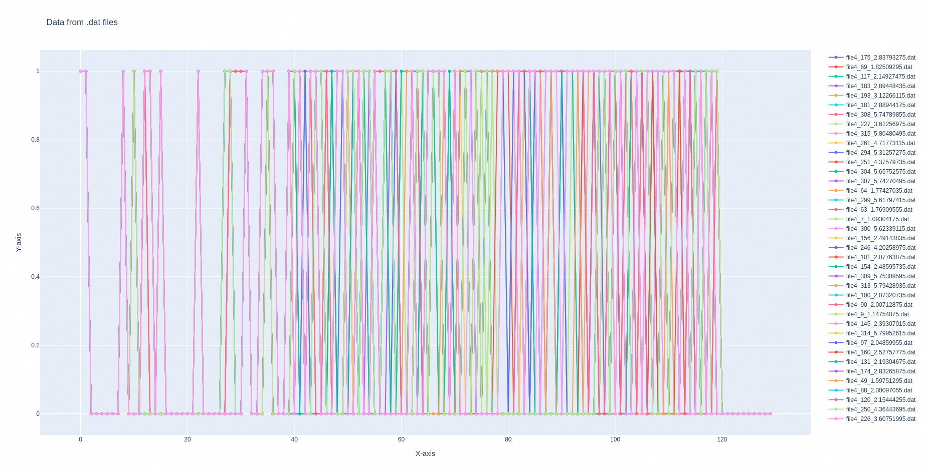
Now, remember that we are acquired these signals with a sample rate of 5 Msps, and the baud rate of ADS-B frames is 1 Mbps, so we need to apply a decimation factor of 5 in order to obtain one sample per bit.

# Decimation factor
decimation_factor = 5

Adding this two modifications to the code, the plot function will be the next.

# Add trace only if data length is sufficient
if len(data) >= samples_per_frame:
    data_sync = synchronize_data(data)
    data_decimate = data_sync[1::decimation_factor]
    trace = go.Scatter(
        x=np.linspace(0, len(data_decimate)-1, len(data_decimate)),
        y=data_decimate,
        mode='lines+markers',
        name=file
    )
    traces.append(trace)

With this script, we will obtain the bit array of the ADS-B frames received.

Decoding Mode-S frame

Now it’s time to decode the frame using pyModeS.First we need to discard the first 8 samples that corresponds with the 8us preamble.Then we are going to retype the data to uint8, reshape the frame to have groups of 4 bits, and finally convert each 4bit packet to hexadecimal..

Finally, using the tell function of the pyModeS package we will obtain the decoded data.

def decode_mode_s(data):
    messages = []
    data = np.asarray(data[8:120])  # Skip the first 8 samples used for synchronization
    bits = (data > 0.5).astype(np.uint8)

    nibbles = bits.reshape(-1,4).tolist()

    weights = np.array([8, 4, 2, 1], dtype=np.uint8)
    vals = (nibbles * weights).sum(axis=1) # Convert 4 bits to a nibble value

    # Lookup table for hex characters
    lut = np.frombuffer(b"0123456789ABCDEF", dtype="S1")
    hex_chars = lut[vals].astype(str)               # array de '0'..'F'
    hex_str = "".join(hex_chars.tolist())

    message = pms.tell(hex_str)

    if message is not None:
        return message
    

If we execute this script from the command line, we will obtain the ICAO address, speed, direction,…

user@host:~/mode-s$ python3 ./data_plot.py 
                     Message: A8000F10D229F1323FD7FE6FFFA9 
                ICAO address: 020139 
             Downlink Format: 21 
                    Protocol: Mode-S Comm-B identity reply 
                 Squawk code: 3061 
                         BDS: BDS60 (Heading and speed report) 
            Magnetic Heading: 230.9765625 degrees
          Indicated airspeed: 248 knots
                 Mach number: 0.8 
        Vertical rate (Baro): -192 feet/minute
         Vertical rate (INS): -64 feet/minute

Conclusions

In this article we decoded ADS-B—going from the 1090 MHz air interface to fully parsed aircraft states using a USRP B206mini-i, a lightweight GNU Radio flowgraph, and the Python pyModeS parser. With a very straightforward process, we extracted positions, velocities, and identifiers from ADS-B messages in just a few lines of code. It’s worth stressing that even portable devices like the B206mini-i or the B205mini-i—plugged into a laptop, paired with a modest antenna and sensible gain/filter settings, are powerful enough to capture and decode a wide variety of signals. Small SDRs plus open-source tools make serious RF analysis accessible, reproducible, and easy to take into the field.